

Introduction
In an earlier blog, I had created a simple model to forecast the long-term (10year) future returns of the Nifty500 using P/B, P/E, and dividend yield as inputs. In the same article, I start with a simplistic model based on the B/P ratio and 10Y future returns of the stocks, and then later I added the E/P and D/P ratios to the model.
I must be honest that I was not too comfortable with the model I had made. Here are reasons why I think so:
The model especially with only B/P as input always predicted positive future returns. Fundamentally, that is wrong. Market returns can be negative, and any decent model must update to capture that.
The constant term was a fixed number. In an ideal world, long-term returns must be factors of things like interest rates, inflation, etc., the model did not bother about them at all.
The model gives a point estimate and assumes that all things in the world do not matter except starting valuations. If life were so predictable stock returns would surely reduce over time. For instance, valuations can stay elevated for a long time, and despite high initial valuation, returns can be good.
So, I had been mulling on how to resolve this and the current blog is an update to the model. The basic idea is borrowed from the article “The Long Run is Lying to You” by Cliff Asness of AQR Capital. This blog tries to improve on that model.
Inputs to the Model
To the model, I add the risk-free rate as an input. Long-term interest bonds are sensitive to interest rates whereas extremely short-term (liquid funds) treasury bills are not so sensitive to interest rates and are more stable and considered “Risk-Free.” RBI database here has risk-free rates. Under Financial Markets ==> Govt Securities Market ==>Weekly ==>Auctions of 91-day Government of India Treasury Bills. The NSE website niftyindices is used to obtain the Nifty500 TRI data over time as well as the P/B, P/E, and Dividend yield data. Other definitions:

The Model
The updated model shall be as follows:

We create a simple X-Y graph in excel to capture this. Excel also computes the predicted regression curve. R2 = 76% is a decent fit.
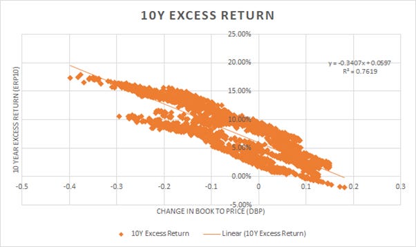
This model is better than the previous model. The way to read and keep it simple is
ERP_10 = -0.34 * dBP + 6%
If there is no change in valuations over time, the 10-year excess returns will be 6%. The way to interpret this is 6% in the long-run excess returns of stocks over risk-free assets in India. This is consistent with data from other countries and is good to see.
It addresses the concerns outlined in the introduction:
The model uses the excess returns to risk-free assets and has a negative slope to valuations. There is a possibility that returns are worse than risk-free assets.
The constant term is the ERP and what we capture now is excess returns to risk-free assets and hence the model is a better fit.
The model provides room for different forecasters to arrive at different numbers based on risk-free asset return forecasts and valuation change and Book price change over time. For example, the long-run returns can increase/decrease based on how the valuations change. An increase in P/B (valuation expansion) will increase the future returns whereas a decrease in P/B (valuation compression) will reduce the future returns.
Also, note that I have tried doing the same exercise with both EP and DP as well. And the R2 for them is poor. The difference of EP is a poor predictor for future returns as well as dividend difference.
Conclusion
We have an updated model which is a combination of change in valuation and risk-free assets returns. The model is a decent fit for usage based on easily available information and does not need the CAPE ratio. Indian stock market Equity Risk Premium is around 6% over risk-free assets.